2  Theory

2.1 LGCP

A Poisson point process is a stochastic set of points indexed in a bounded n-dimensional space, where the number of points in the set is a Poisson distributed random variable. The LGCP extends the process by explicitly incorporating spatial or temporal correlation into the definition of the intensity of the process. Diggle et al. (2013) is a good reference for these type of models. I’ll give some details below, and then discuss the INLA approach for actually estimating the model.

The NHPP is characterized by an intensity that can be defined as the expected number of observations per unit area. For a given region \(A\), the number of individuals occurring within the region will be Poisson distributed. The mean of the distribution can be defined by the integral of the intensity over the region: \[ \Delta(A) = \int_A \lambda(s)ds. \] Sadly, the intensity is an unobservable and unknown process, and therefore must be modelled as a function of covariates. The intensity takes the general parameterization as \[ \lambda(s) = \exp[\alpha + \beta'x(s)]. \] In the previous blog I discussed incorporating sampling bias, but I will leave that out now. Some version of this will come back when discussing preferential sampling.

Now, in the LGCP we incorporate a Gaussian Random Field (also described as Gaussian spatial field, spatial random effect, or latent spatial field. I’m not sure exactly when the difference in description leads to a distinctly different spatial model) to incorporate spatial correlation in the model of intensity. \[ \lambda(s) = \exp[\alpha + \beta'x(s) + f_s(s)]. \] The spatial effect is denoted as \(f_s(s)\) in order to distinguish from temporal contributions. \(f_s(s)\) can be thought of as a continuous spatial effect that is evaluated at certain locations.

The main thing is that, once we incorporate \(f_s(s)\), we are forced to use a covariance structure that depends on the resolution of the grid or mesh that will be used to approximate the continuous spatial effect. Furthermore, we are still stuck with the problem of an intractable integral in the likelihood of the LGCP (as in the case of the Poisson process). Thus, the computational complexity makes this approach prohibitively costly when using MCMC approaches to estimate the model in any region of practical interest. Hence, other approximations to the posterior of the parameters in the LGCP are necessary.

2.2 INLA

The Integrated Nested Laplace Approximation has been proposed by Rue, Martino, and Chopin (2009) as a fast way to estimate the posterior of models with latent Gaussian structure. The LGCP is certainly an instance of models of this class. In the following description of the model, I present it nearly identically to the original paper, and/or from other well-done sources, including:

1. https://becarioprecario.bitbucket.io/spde-gitbook really has a lot of detail, specifically for the SPDE innovation to INLA.
2. https://becarioprecario.bitbucket.io/inla-gitbook/ch-INLA.html is also good for focusing just on INLA.
3. The book of Paula Moraga https://www.paulamoraga.com/book-spatial/sec-geostatisticaldataSPDE.html is concise and clear for an initial tutorial, though not as detailed.
4. This book is also a very good resource: Spatial and Spatio-temporal Bayesian Models with R-INLA. Blangiardo, Marta, and Michela Cameletti. 2015.

There is nothing new under the sun here. I’m just condensing some resources for my own reference. So, taking notation directly from the Rue paper, INLA is concerned with models with an additive predictor that takes the general form \[ \eta_i = \alpha + \sum^{n_f}_{j=1}f^{(j)}(u_{ij}) + \sum^{n_{\beta}}_{k=1} \beta_kz_{ki} + \epsilon_i, \] where \(\alpha\) is an intercept, \(f\) are unknown functions of \(\mathbf{u}\), \(\beta\) are the typical fixed effects for covariates \(\mathbf{z}\), and \(\epsilon_i\) is the additional noise in the process. Additionally, \(\mathbf{x}\) will refer to the vector of latent Gaussian variables (Gaussian by definition of the prior), and \(\boldsymbol{\theta}\) the vector of hyperparameters that we usually deal with in a Bayesian model. These need not be inherently Gaussian. In the book of Blangiardo and Cameletti (2015), the hyperparameters and latent field are denoted by \(\psi\) and \(\theta\) respectively, which is clearer than using \(\mathbf{x}\) to describe the latent field, but here I’m sticking to the original notation.

Still taking from the notation of the Rue paper, the joint posterior of hyperparameters and latent variables is written as \[ \begin{aligned} \pi(\mathbf{x},\mathbf{\theta}|\mathbf{y})\propto\pi(\mathbf{\theta})\pi(\mathbf{x}|\mathbf{\theta})\prod_{i\in I}\pi(y_i|x_i,\mathbf{\theta})\\ \propto\pi(\mathbf{\theta})|Q(\mathbf{\theta})|^{1/2}\exp\bigg[-\frac{1}{2}\mathbf{x}^TQ(\mathbf{\theta})\mathbf{x}+\sum_{i\in I}\log\{\pi(y_i|x_i,\mathbf{\theta})\}\bigg], \end{aligned} \] where \(\pi(y_i|x_i,\mathbf{\theta})\) is the distribution of the response variable and \(|Q(\mathbf{\theta})|^{1/2}\exp\bigg[-\frac{1}{2}\mathbf{x}^TQ(\mathbf{\theta})\mathbf{x}\bigg]\) is the Gaussian prior on the GRMF with a mean of 0 and precision matrix \(Q\), conditional on \(\mathbf{\theta}\).

The main point of INLA is to make approximations of the posterior marginals of the hyperparameters and (even more importantly) the latent field. The posterior marginal of one component of the hyperparameters is \[ \pi(\theta_j|\mathbf{y}) = \int \pi(\mathbf{\theta}|\mathbf{y})d\mathbf{\theta}_{-j}. \] Notice the \(-j\) components are integrated out. The posterior marginal of a component of the latent field is \[ \pi(x_i|\mathbf{y}) = \int \pi(x_i|\mathbf{\theta},\mathbf{y})\pi(\mathbf{\theta}|\mathbf{y})d\mathbf{\theta}, \] again, sticking to the \(\mathbf{x}\) notation.

Following the procedure of INLA, first \(\pi(\theta|y)\) will need to be approximated, and then \(\pi(x_i|\theta,y)\). The integration over \(\pi(x_i|y)\) will be done numerically, using points from (|y). The approximations themselves are done with the Laplace Approximation, or a Gaussian-type approximation. To approximate the first quantity, \(\pi(\theta|y)\), a Laplace approximation is used from Tierney and Kadane, 1986: \[ \tilde{\pi}(\theta|y) \propto \frac{\pi(x,\theta,y)}{\tilde{\pi}_G(x|\theta,y)}\bigg|_{x=x^*(\theta)} = \frac{\pi(y|x,\theta)\pi(x|\theta)\pi(\theta)}{\tilde{\pi}_G(x|\theta,y)}\bigg|_{x=x^*(\theta)}, \] where \(x^*(\theta)\) refers to the mode of \(\tilde{\pi}_G(x|\theta,y)\). As per the name, IN(ested)LA, this approximation uses a NESTED approximation, \(\tilde{\pi}_G(x|\theta,y)\). \(\tilde{\pi}_G\) is the Gaussian approximation to the latent field, which works because we already know the latent field to be prior-ly distributed as Gaussian. In fact, the contribution of this paper is to then to improve on the approximation of \(\pi(x_i|\theta, y)\) with another approximation, the Laplace Approximation (LA), beyond just a simple Gaussian. The paper discusses 3 approximations to \(\pi(x_i|\theta, y)\): the Gaussian, LA, and a simplified LA.

The LA approximation is written as \[ \tilde{\pi}_{LA}(x_i|\theta,y) \propto \frac{\pi(x,\theta,y)}{\tilde{\pi}_{GG}(x_{-i}|x_i,\theta,y)}\bigg|_{x_{-i}=x^*_{-i}(x_i,\theta)}, \] where \(x^{*}_{-i}(x_i,\theta)\) is the mode of \(\tilde{\pi}_{GG}(x_{-i}|x_i,\theta,y)\). This approximation can be computationally intensive since it is necessary to recompute \(\tilde{\pi}_{GG}(x_{-i}|x_i,\theta,y)\) for each element of \(x\) and \(\theta\).

Once the approximations of \(\tilde{\pi}(\theta|y)\) of \(\tilde{\pi}(x_i|\theta,y)\) are found, the marginals for each element \(x_i\) can be approximated:

\[ \tilde{\pi}(x_i|y) \approx\sum\tilde{\pi}(x_i|\theta^{(i)},y)\tilde{\pi}(\theta^{(j)}|y)\Delta_j, \] for integration points \(\theta^{(i)}\) which are found by the exploration of the posterior for \(\theta\). This is done in a few different ways, for example by creating a standardized \(Z\) variable around the mode and inverse hessian of \(\log \tilde{\pi}(\theta|y)\). There are quite a few more details to this part that I won’t discuss here, but may come up when up using the INLA software itself (choosing the integration scheme, for instance).

From the math above it is not possible to fully understand the INLA approach, but it should enough of a technical description to understand the main ideas (approximate the hyperparameters and latent conditionals, then numerically integrate to approximate the marginals).

2.3 SPDE connection

The Stochastic Partial Differential Equation (SPDE) approach is an innovation from Lindgren, Rue, and Lindström (2011) on the INLA method. The approach allows the representation of a continuous Gaussian Field with a Gaussian Markov Random Field. The connection to the Rue, Martino, and Chopin (2009) paper is that Lindgren, Rue, and Lindström (2011) connected the GRMF models of INLA to specific (continuous) GFs. As spatial statisticians, we care about the continuous case more than approximations in discrete space, and SPDE connected the two.

To be slightly more specific, it turns out a GF with Matern covariance is a solution to a specific SPDE. The solution to the SPDE is found via a set of basis functions defined on a triangulation of the spatial region. The resulting GRMF is an approximation to the SPDE. So this approach allows us to approximate the solution of the SPDE with a GRMF that corresponds to a specific GF with matern covariance.

2.3.1 Mesh

In the SPDE approach a triangulated mesh (the finite element representation) is used to approximate the solution to the SPDE using spatial weights defined at the vertices of the mesh. \[ x(u) = \sum^n_{k=1}\psi_k(u)w_k, \] where \(w_k\) are Gaussian weights and \(\psi_k\) are the piecewise linear basis functions, and \(n\) is the number of vertices in the entire triangulation of the domain. This means that the weights represent the values of the field at each vertex, and the basis functions are used to interpolate the value of the observation in the interior of the triangle, where \(\psi_k(u)=1\) only at vertex \(k\) of the triangle containing \(u\). A result of Lindgren, Rue, and Lindström (2011) is to show that the weights follow a GRMF and to derive the precision matrix.

The practical implication of this the SPDE approach is that you will need to define the mesh before modelling. The results will be sensitive to this choice, so it is important to explore the impact of the mesh on the model estimation. I’ll show this a little once I get to the coding.

In INLA software, a projection matrix maps the GMRF from the observations to the triangulation nodes. The observation will be represented as the weighted average using the weights and values from the triangulation and projection matrix. For example, in the picture below, for observation \(s\) the value Z\((s)\) is calculated as \(Z(s)\approx \frac{T_1}{T}Z_1+\frac{T_2}{T}Z_2+\frac{T_3}{T}Z_3\). This figure is taken from https://www.paulamoraga.com/book-spatial/sec-geostatisticaldataSPDE.html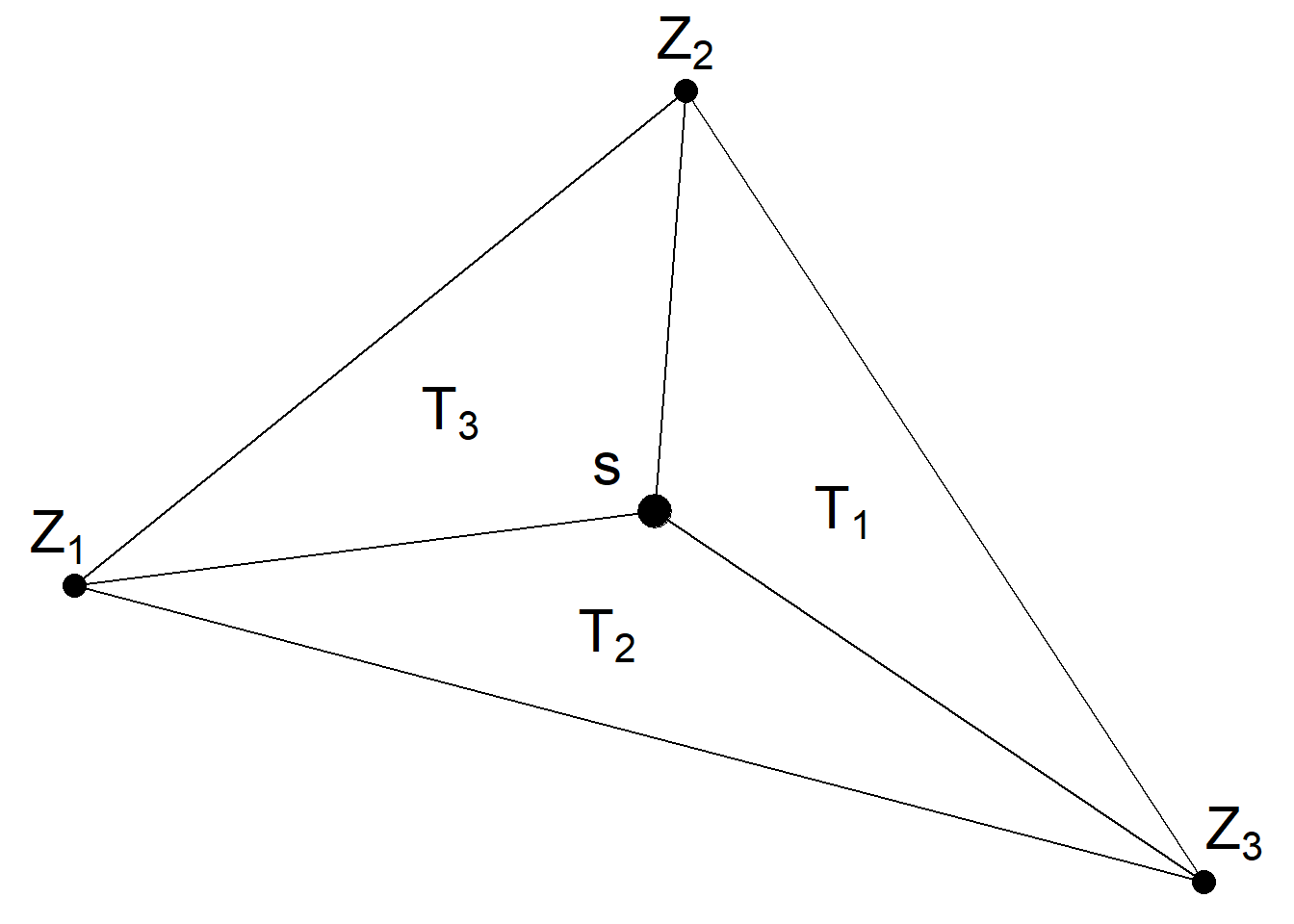

2.3.2 Off the grid

Simpson et al. (2016) developed an approach for approximating the likelihood of the LGCP within the INLA and SPDE framework, using a finite-dimensional random field \[ Z(s) = \sum^n_{i=1}z_i\phi_i(s), \] where \(z=(z_1...,z_n)^T\) is a multivariate Gaussian vector and \(\{\phi_i(s)\}^n_{i=1}\) is a set of basis functions. Using the random field, they propose an approximation to the LGCP that does not rely on the discretization of the domain into a grid. Furthermore, they are able to leverage the triangulation of the SPDE approach to compute the LGCP likelihood when using their random field approximation. The implication of this for our LGCP modelling is that the INLA framework can conveniently be used approximate to the LGCP likelihood and posterior.

2.4 In conclusion…

That was a bit of a longer-than-intended dive into INLA. But INLA is a more mathematically complicated method than other approximations, and I wanted to solidify the details for myself. It’s not always that way, sometimes it’s nice just to jump straight into the application, but with INLA it seemed prudent to pick over the details. Now, onto using the software with some of my own data and use-cases. I’ll now proceed to discuss the modelling procedure using INLA and inlabru. I’ll compare the software and details of the implementation, first for a continuous measurement and then for point data using an LGCP.

Blangiardo, Marta, and Michela Cameletti. 2015. Spatial and Spatio-Temporal Bayesian Models with r-INLA. John Wiley & Sons, Ltd. https://doi.org/https://doi.org/10.1002/9781118950203.

Diggle, Peter J., Paula Moraga, Barry Rowlingson, and Benjamin M. Taylor. 2013. “Spatial and Spatio-Temporal Log-Gaussian Cox Processes: Extending the Geostatistical Paradigm.” Statistical Science 28 (4): 542–63. https://doi.org/10.1214/13-STS441.

Lindgren, Finn, Håvard Rue, and Johan Lindström. 2011. “An Explicit Link Between Gaussian Fields and Gaussian Markov Random Fields: The Stochastic Partial Differential Equation Approach.” Journal of the Royal Statistical Society: Series B (Statistical Methodology) 73 (4): 423–98. https://doi.org/10.1111/j.1467-9868.2011.00777.x.

Rue, Håvard, Sara Martino, and Nicolas Chopin. 2009. “Approximate Bayesian Inference for Latent Gaussian Models by Using Integrated Nested Laplace Approximations.” Journal of the Royal Statistical Society: Series B (Statistical Methodology) 71 (2): 319–92. https://doi.org/10.1111/j.1467-9868.2008.00700.x.

Simpson, D., J. B. Illian, F. Lindgren, S. H. Sørbye, and H. Rue. 2016. “Going Off Grid: Computationally Efficient Inference for Log-Gaussian Cox Processes.” Biometrika 103 (1): 49–70. https://doi.org/10.1093/biomet/asv064.