4  Implementation of LGCP in INLA and INLABRU

4.1 INLA

Having completed air pollution modelling in INLA and inlabru, it is time to move on to the LGCP and the point process model. A couple of online resources about point process modelling in INLA include: https://becarioprecario.bitbucket.io/spde-gitbook/ch-stapp.html#sec:burkitt and https://www.paulamoraga.com/book-spatial/point-process-modeling.html. I’ll again be relying on the Moraga book for template code.

The model fit here has intensity specified as \[ \lambda(s) = \exp[\beta_0 + f(s)]. \] Here I only use an intercept and spatial field to model the intensity, so we won’t have to worry about downloading any covariates.

library(INLA)
library(inlabru)
library(sf)
library(ggplot2)
library(viridis)
library(terra)
library(tidyterra)
library(dplyr)
library(readr)
library(rasterVis)

Now for the data. I’ll use butterfly data from citizen science observations made in the Netherlands in 2023. The data is available in the GBIF repository https://doi.org/10.15468/dl.p5cy6n, which includes all butterfly observations uploaded to observation.org. So it’s necessary to filter the dataset down to just the Netherlands. I also filter for the species Lasiommata megera.

Here is a nice picture (Charles J. Sharp - Own work, from Sharp Photography, sharpphotography.co.uk, CC BY-SA 4.0, https://commons.wikimedia.org/w/index.php?curid=81510351):

Once the filtering is done, we are left with 2705 observations.

file_name <- file.path("D:", "data", "gbif_observation_org_butterflies", "gbif_butterfly_observation-org", "gbif_subset_netherlands_lepidoptera.csv")
d <- read_delim(file_name, delim='\t', col_types=cols(infraspecificEpithet=col_character()))
d %>% filter(species=="Lasiommata megera") -> d
dim(d)

[1] 2705   50

d <- st_as_sf(d, coords = c("decimalLongitude", "decimalLatitude"))
st_crs(d) <- "EPSG:4326"
#projMercator <- "+proj=merc +a=6378137 +b=6378137 +lat_ts=0 +lon_0=0
#+x_0=0 +y_0=0 +k=1 +units=km +nadgrids=@null +wktext +no_defs"
projMercator <- st_crs("EPSG:3857")$proj4string
# Observed coordinates
d <- st_transform(d, crs = projMercator)

Before, I used the Netherlands map directly, but now there is some extra processing to do, due to little isolated boundaries within the main polygon of the Netherlands border.

layers <- st_layers(file.path("D:", "data", "maps", "netherlands_bestuurlijkegrenzen_2021", "bestuurlijkegrenzen.gpkg"))
#print(str(layers))
map <- st_read(file.path("D:", "data", "maps", "netherlands_bestuurlijkegrenzen_2021", "bestuurlijkegrenzen.gpkg"), layer = "landsgrens")

Reading layer `landsgrens' from data source 
  `D:\data\maps\netherlands_bestuurlijkegrenzen_2021\bestuurlijkegrenzen.gpkg' 
  using driver `GPKG'
Simple feature collection with 1 feature and 2 fields
Geometry type: MULTIPOLYGON
Dimension:     XY
Bounding box:  xmin: 10425.16 ymin: 306846.2 xmax: 278026.1 ymax: 621876.3
Projected CRS: Amersfoort / RD New

map <- st_union(map)
map <- st_as_sf(map)
# there's a little isolated spec in the map!
border_polygon <- st_cast(map, "POLYGON")
border_polygon <- st_as_sfc(border_polygon)
geos <- lapply(border_polygon, function(x) x[1])
#for (g in geos){
#  plot(st_polygon(g))
#}
# Get the border polygon
border_final <- st_polygon(geos[[1]])
# We still need sf object
border_final <- st_sfc(border_final, crs=st_crs(map))
border_final <- st_as_sf(border_final)
plot(border_final)

map <- border_final
map <- st_transform(map, crs = projMercator)
coo <- st_coordinates(d)
ggplot() + geom_sf(data = map) +
  geom_sf(data = d) + coord_sf(datum = projMercator)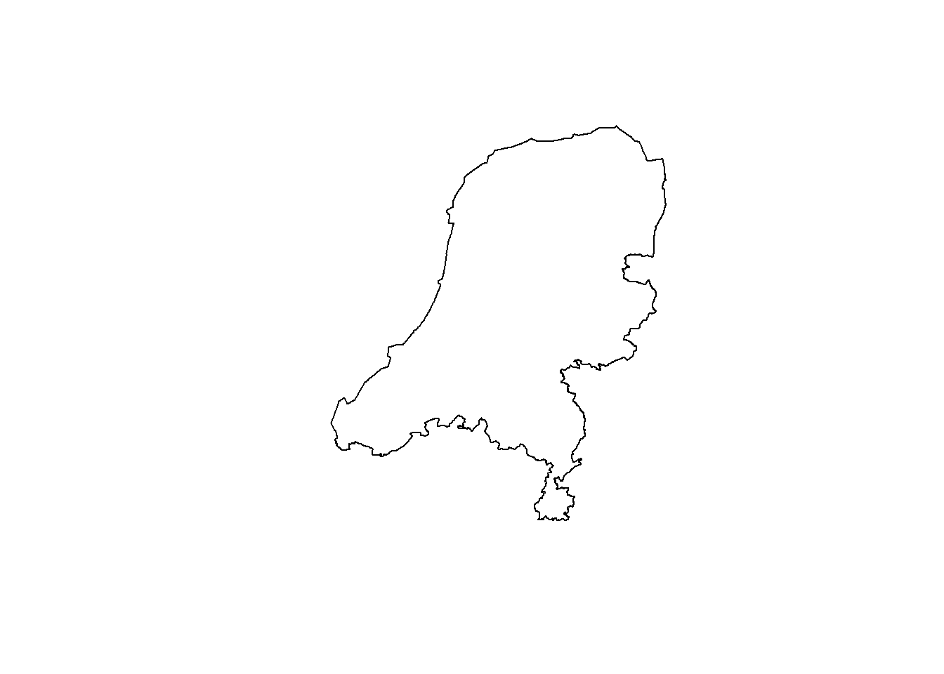

# Save this for later
st_write(map, file.path("D:", "data", "maps", "netherlands_bestuurlijkegrenzen_2021", "clean_nl_boundary.gpkg"), append=F)

Deleting layer `clean_nl_boundary' using driver `GPKG'
Writing layer `clean_nl_boundary' to data source 
  `D:/data/maps/netherlands_bestuurlijkegrenzen_2021/clean_nl_boundary.gpkg' using driver `GPKG'
Writing 1 features with 0 fields and geometry type Polygon.

So that gives us a very clean map, with the location of Lasiommata megera observations.

As in the previous example for air pollution data, we again create prediction points across the spatial region. These will be the locations at which the intensity is predicted.

# raster grid covering map
grid <- terra::rast(map, nrows = 50, ncols = 50)
# coordinates of all cells
xy <- terra::xyFromCell(grid, 1:ncell(grid))
# transform points to a sf object
dp <- st_as_sf(as.data.frame(xy), coords = c("x", "y"),
               crs = st_crs(map))

# indices points within the map
indicespointswithin <- which(st_intersects(dp, map,
                                           sparse = FALSE))

# points within the map
dp <- st_filter(dp, map)

ggplot() + geom_sf(data = map) +
  geom_sf(data = dp) + coord_sf(datum = projMercator)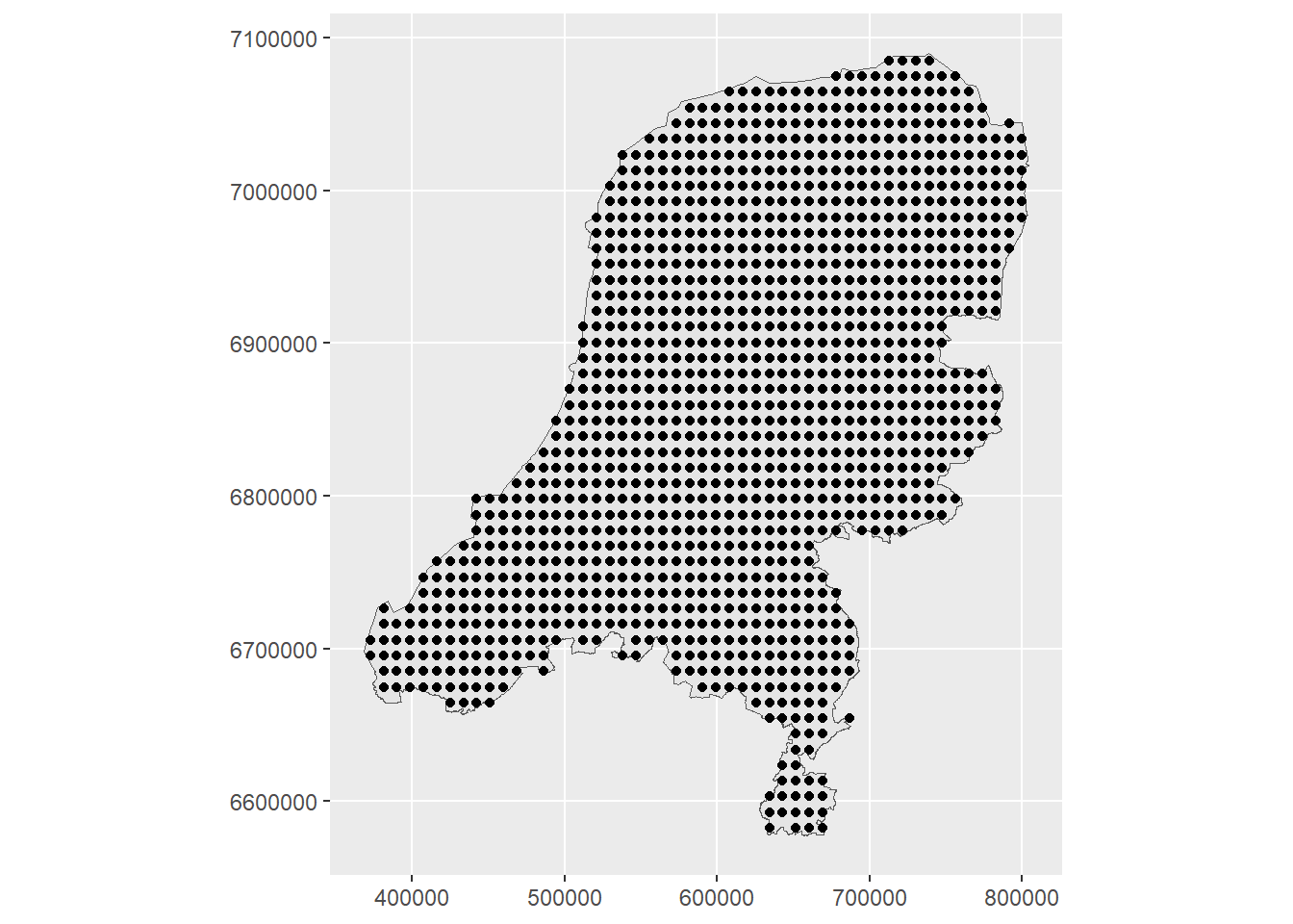

coop <- st_coordinates(dp)

Next, build the mesh. I left the projection in meters here, so the max.edge has to reflect those units. I also found that the parameter estimates in this example were particularly sensitive to the resolution of the triangles in the mesh, so I chose a max.edges that gave good estimates but also weren’t too slow in the fitting process. The main takeaway here is that it is important to explore different meshes a bit and the effect of that on your model.

loc.d <- cbind(st_coordinates(map)[, 1], st_coordinates(map)[, 2])
mesh <- inla.mesh.2d(loc.domain = loc.d, max.edge = c(30000, 50000), crs=crs(d))
plot(mesh)
points(coo, col = "red")
axis(1)
axis(2)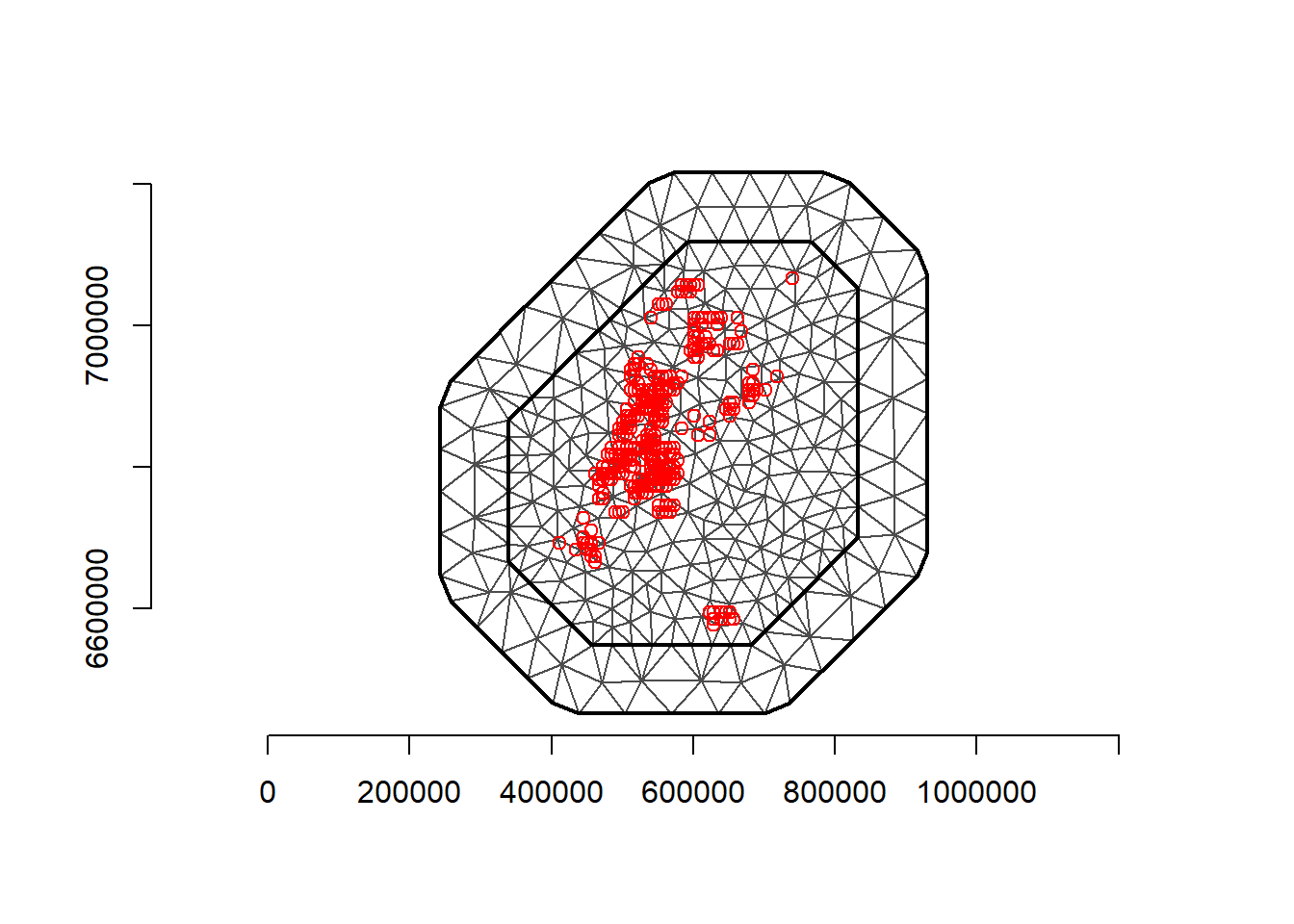

(nv <- mesh$n)

[1] 886

(n <- nrow(coo))

[1] 2705

Using spde <- inla.spde2.matern(mesh = mesh, alpha = 2, constr = TRUE) led to some differences in the inla and INLABRU models, mainly in that the intercept was quite different between the two. So I started to use the Penalized Complexity priors on the matern function instead. The PC priors can be read about in Daniel Simpson et al. (2017). prior.range\(=(\rho\),\(p_{\rho})\) specifies \(P(\rho < \rho_0)=p_ρ\), the probability that the range is less than a certain amount \(\rho_0\). This indicates how likely it is that the spatial range of the field degrades quickly. The same can be said for prior.sigma, only for the marginal standard deviation of the field.

spde <- inla.spde2.pcmatern(mesh = mesh, alpha = 2, constr = TRUE, prior.range = c(10, 0.1), prior.sigma = c(1, 0.01))

In the point process setting, it is necessary to use the method of D. Simpson et al. (2016). This uses a dual mesh to approximate the point process likelihood. It is called a dual mesh because a mesh of polygons is generated, each centered around the vertices of the triangles in the first mesh. The code to create the dual mesh is available in both the SPDE book and Moraga book.

book.mesh.dual <- function(mesh) {
    if (mesh$manifold=='R2') {
        ce <- t(sapply(1:nrow(mesh$graph$tv), function(i)
            colMeans(mesh$loc[mesh$graph$tv[i, ], 1:2])))
        library(parallel)
        pls <- mclapply(1:mesh$n, function(i) {
            p <- unique(Reduce('rbind', lapply(1:3, function(k) {
            j <- which(mesh$graph$tv[,k]==i)
            if (length(j)>0) 
            return(rbind(ce[j, , drop=FALSE],
            cbind(mesh$loc[mesh$graph$tv[j, k], 1] +
            mesh$loc[mesh$graph$tv[j, c(2:3,1)[k]], 1], 
            mesh$loc[mesh$graph$tv[j, k], 2] +
            mesh$loc[mesh$graph$tv[j, c(2:3,1)[k]], 2])/2))
            else return(ce[j, , drop=FALSE])
            })))
            j1 <- which(mesh$segm$bnd$idx[,1]==i)
            j2 <- which(mesh$segm$bnd$idx[,2]==i)
            if ((length(j1)>0) | (length(j2)>0)) {
            p <- unique(rbind(mesh$loc[i, 1:2], p,
            mesh$loc[mesh$segm$bnd$idx[j1, 1], 1:2]/2 +
            mesh$loc[mesh$segm$bnd$idx[j1, 2], 1:2]/2, 
            mesh$loc[mesh$segm$bnd$idx[j2, 1], 1:2]/2 +
            mesh$loc[mesh$segm$bnd$idx[j2, 2], 1:2]/2))
            yy <- p[,2]-mean(p[,2])/2-mesh$loc[i, 2]/2
            xx <- p[,1]-mean(p[,1])/2-mesh$loc[i, 1]/2
            }
            else {
            yy <- p[,2]-mesh$loc[i, 2]
            xx <- p[,1]-mesh$loc[i, 1]
            }
            Polygon(p[order(atan2(yy,xx)), ])
        })
        return(SpatialPolygons(lapply(1:mesh$n, function(i)
            Polygons(list(pls[[i]]), i))))
    }
    else stop("It only works for R2!")
}
dmesh <- book.mesh.dual(mesh)
plot(dmesh)
axis(1)
axis(2)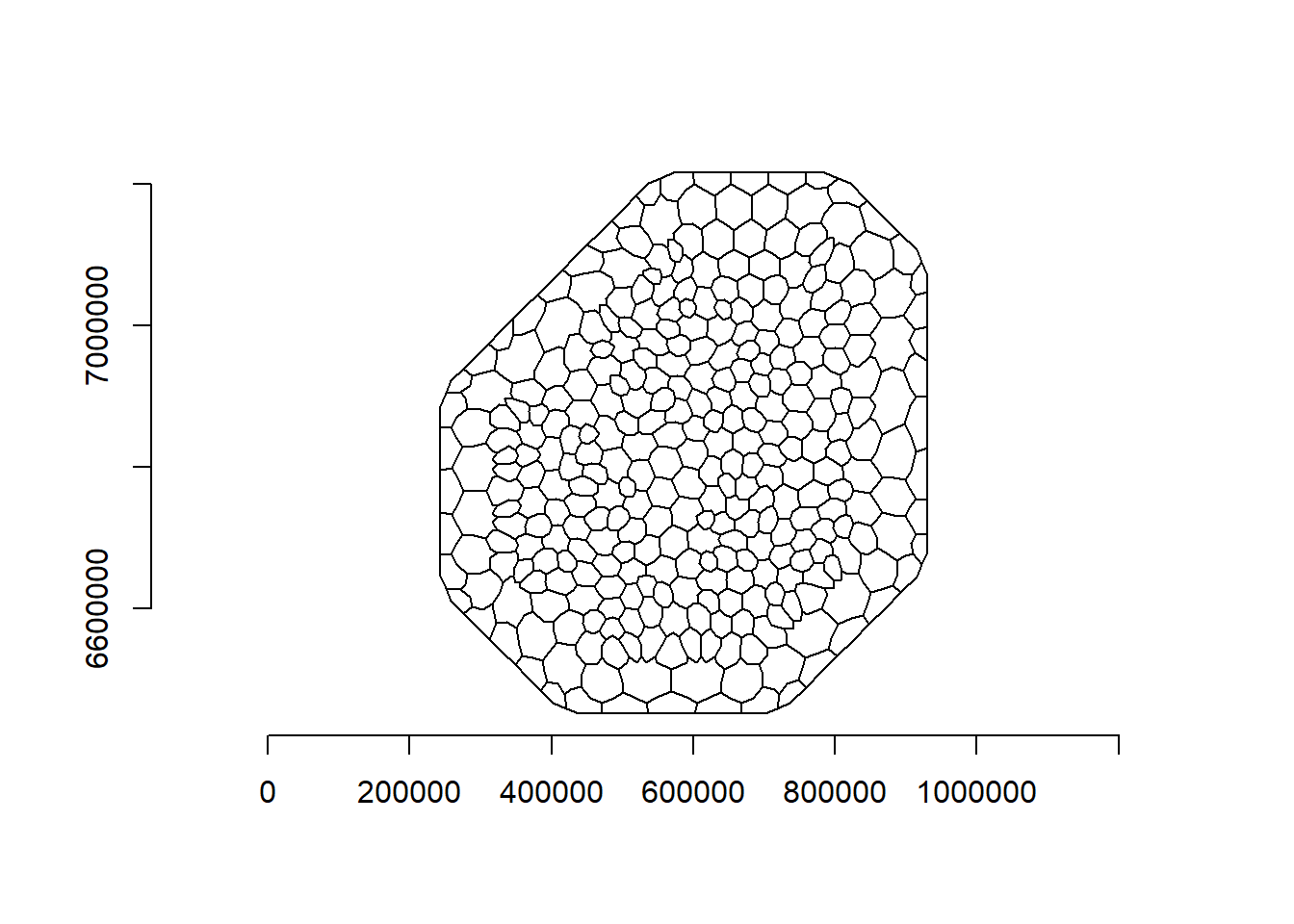

We then do something a little tricky. The mesh is larger than the domain that the points were observed in or the study region. So the intersections between the polygons in the mesh and the locations in \(D\) are computed and the integration weights are returned based on the overlap.

domain.polys <- Polygons(list(Polygon(loc.d)), '0')
domainSP <- SpatialPolygons(list(domain.polys))
domain_sf <- st_as_sf(domainSP)
domain_sf <- st_set_crs(domain_sf, projMercator)
mesh_sf <- st_as_sf(dmesh)
mesh_sf <- st_set_crs(mesh_sf, projMercator)
# Check if the mesh polygons overlap with any of the locations 
w <- sapply(1:length(dmesh), function(i) {
  if(length(st_intersects(mesh_sf[i,], domain_sf)[[1]])>0){
    return(sf::st_area(sf::st_intersection(mesh_sf[i, ], domain_sf)))
  }
  else return(0)
})

# Fun little exercise as an alternative way to calculate the weights.
# dp <- fm_pixels(mesh, dims = c(50, 50), mask = domain_sf)
# # Project mesh basis functions to pixel locations and multiply by pixel weights 
# # Sum these contributions for each basis function 
# A_pixels <- fm_basis(mesh, loc = dp)
# pixel_weights <- st_area(dp)
# pixel_weights <- as.numeric(pixel_weights)
# A_weighted <- Diagonal(length(pixel_weights), pixel_weights) %*% A_pixels
# w <- Matrix::colSums(A_weighted)
# w <- as.vector(w)
# sum(w)

sum(w)

[1] 111060620373

st_area(map)

111060620373 [m^2]

Notice that the weights and and the area of the domain are the same.

We can see in the plot below that we are left with a very nice looking mesh, where the black integration points fall within the Netherlands domain and red fall outside of it.

plot(mesh)
plot(domain_sf, add=T)
points(mesh$loc[which(w > 0), 1:2], col = "black", pch = 20)
points(mesh$loc[which(w == 0), 1:2], col = "red", pch = 20)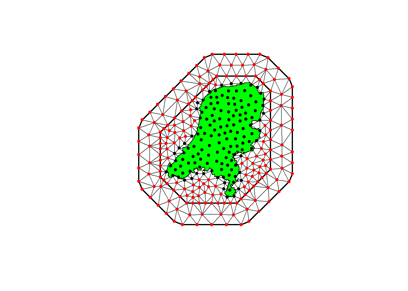

Next, create the INLA stack, for both observations and for prediction points. In the first section I didn’t provide that much detail about the stack, so I’ll explain it in more detail here.

First we create vectors for the observed response and for estimation. For y.pp, nv is the number of mesh nodes and n is the number of observations, where there will be a 0 for each element of length nv and a 1 for each of length n. e.pp will consist of the integration weights w of length nv and a set of 0s of length n. This is for the numerical integration in the LGCP likelihood. Just as in the point process likelihood, we have two components: An intractable integral to be approximated, and a product of point locations: \[ L(\lambda)\propto\prod_iλ(s_i​)\exp\left(−\int_D\lambda(s)ds\right). \]

y.pp <- rep(0:1, c(nv, n))
length(y.pp)

[1] 3591

e.pp <- c(w, rep(0, n))
length(e.pp)

[1] 3591

Next set up the projection matrix. This will be used to compute the linear predictor, generally written \[ \boldsymbol{\eta} = \boldsymbol{1}\beta_0 + \boldsymbol{Az}. \] where \(\boldsymbol{z}=\{z_1,z_2,,,z_{n_v}\}\) will be the values of the spatial field at the nodes.

In the model here, we have both nodes and observed locations, \(\boldsymbol{z}=\{z_1,z_2,,,z_{n_v}, z_{{n_v+1}}, ...,z_{n_v+n}\}\), and the points for prediction, \(\boldsymbol{z}_{pred}=\{z_1,z_2,,,z_{n_{pred}}\}\). So we can write that all out as \[ \begin{aligned} \begin{pmatrix} \boldsymbol{\eta}_{node} \\ \boldsymbol{\eta}_{obs} \end{pmatrix} &= \begin{pmatrix} \boldsymbol{1}_{n_v}\\ \boldsymbol{1}_n \end{pmatrix}\beta_0 + \begin{pmatrix} \boldsymbol{A}_{n_v}\\ \boldsymbol{A}_n \end{pmatrix}\boldsymbol{z}\\ \boldsymbol{\eta}_{npred} &= \boldsymbol{1}_{npred} \beta_0 + \boldsymbol{A}_{npred} \boldsymbol{z}_{pred} \end{aligned}, \] so that there is a response for each component, an intercept for each, and a projection matrix for each. The below code reflects this. Notice that for A.y and A.pp, we use the function inla.spde.make.A(). This function interpolates the values of the spatial field at the observed location using the triangles in the mesh that each location falls within.

# Projection matrix for the integration points 
# It is diagonal here because the values of the mesh vertices are the integration points themselves.
A.int <- Diagonal(nv, rep(1, nv))
# matrix for observed points 
A.y <- inla.spde.make.A(mesh = mesh, loc = coo)
# matrix for mesh vertices and locations
A.pp <- rbind(A.int, A.y)

# We also create the projection matrix Ap.pp for the prediction locations.
Ap.pp <- inla.spde.make.A(mesh = mesh, loc = coop)

Then create the stacks themselves. We provide the response and estimation vectors to the data argument and the A projection matrices to the A argument. The effect argument takes the intercept and the index of spatial effects. If we had covariates, this is where we would provide them, also in a list.

# stack for estimation
stk.e.pp <- inla.stack(tag = "est.pp",
data = list(y = y.pp, e = e.pp), 
A = list(1, A.pp),
effects = list(list(b0 = rep(1, nv + n)), list(s = 1:nv)))

# stack for prediction stk.p
stk.p.pp <- inla.stack(tag = "pred.pp",
data = list(y = rep(NA, nrow(coop)), e = rep(0, nrow(coop))),
A = list(1, Ap.pp),
effects = list(data.frame(b0 = rep(1, nrow(coop))),
               list(s = 1:nv)))

# stk.full has stk.e and stk.p
stk.full.pp <- inla.stack(stk.e.pp, stk.p.pp)

Finally, we can fit the model. This looks about the same as in the continuous setting. Notice the different strategy options for both the integration strategy and for the posterior approximation itself. control.predictor returns the posterior marginals for the observed and node locations, with link=1 using the same link function as given in family = 'poisson' earlier.

formula <- y ~ -1 + b0 + f(s, model = spde)
res <- inla(formula,  family = 'poisson',
  data = inla.stack.data(stk.full.pp),
  control.inla=list(int.strategy = 'grid', strategy="adaptive"),
  control.predictor = list(compute = TRUE, link = 1,
    A = inla.stack.A(stk.full.pp)),
    E = inla.stack.data(stk.full.pp)$e,
  control.fixed=list(prec = 0.001))

prec = 0.001 sets a vague Gaussian prior, \(N(0, \sigma^2=1/\text{prec})\).

We can check the estimate for the intercept, as well as the parameters for the spatial field.

res$summary.fixed

        mean         sd 0.025quant  0.5quant 0.975quant      mode kld
b0 -17.53066 0.01922714  -17.56835 -17.53066  -17.49298 -17.53066   0

res$summary.hyperpar

                   mean          sd 0.025quant   0.5quant 0.975quant       mode
Range for s 106.7471710 263.8429977 7.25852152 42.6774769 619.967476 14.9620415
Stdev for s   0.3656843   0.4412572 0.03915794  0.2339294   1.508595  0.1009712

Then extract the predictions.

index <- inla.stack.index(stk.full.pp, tag = "pred.pp")$data
pred_mean <- res$summary.fitted.values[index, "mean"]
pred_ll <- res$summary.fitted.values[index, "0.025quant"]
pred_ul <- res$summary.fitted.values[index, "0.975quant"]
grid$mean <- NA
grid$ll <- NA
grid$ul <- NA

grid$mean[indicespointswithin] <- pred_mean
grid$ll[indicespointswithin] <- pred_ll
grid$ul[indicespointswithin] <- pred_ul

And plot the predicted intensity

#levelplot(raster::brick(grid), layout = c(3, 1),
#names.attr = c("Mean", "2.5 percentile", "97.5 percentile"))
# Ah that looks good! There is some numerical problem, or my predictions are on the wrong scale.
min_val <- global(log(grid$mean), "min", na.rm = TRUE)[[1]]
max_val <- global(log(grid$mean), "max", na.rm = TRUE)[[1]]
ggplot() +
  geom_spatraster(data = log(grid$mean)) +
  labs(title = "Predicted intensity on log linear scale",
       fill = "Intensity") +
  scale_fill_viridis_c(limits=c(min_val, max_val), breaks = seq(min_val, max_val, length.out = 10)) +
  theme_minimal()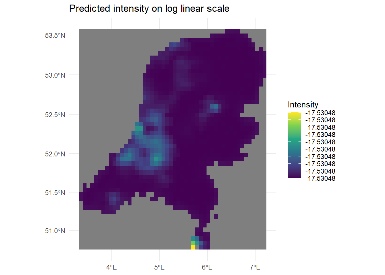

We can see in the legend that the intensity changes must be very small, because even on the log scale the legend values do not change. This is discussed more in the next section.

4.2 Inlabru

Next: Inlabru. Firstly, we have to make sure to get the domain for the sampler correct. The INLA code does it above, but inlabru by default does not. More about that here https://inlabru-org.github.io/inlabru/articles/2d_lgcp_plotsampling.html and actually the exact problem here: https://groups.google.com/g/r-inla-discussion-group/c/0bBC9bVV-L4 even though the problem was with preferential sampling. We had already done this in the code above to get the domain correct for INLA. Even with including sampler=domain_sf here, the estimates are not exactly the same as INLA, but closer than it was before.

ips <- fm_int(
  domain = list(geometry = mesh),
  samplers = domain_sf
)

ggplot() +
  geom_fm(data = mesh) +
  gg(ips, aes(size = weight)) +
  scale_size_area(max_size = 1)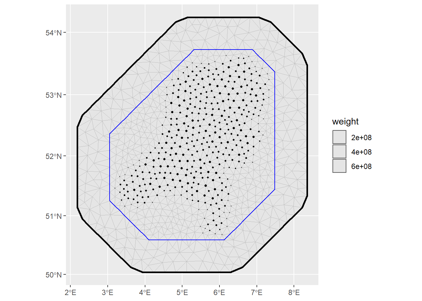

Then fit the inlabru model and check the summary output:

formula_inlabru <- geometry ~ -1 + b0(1) + f(geometry, model = spde)
fit1 <- lgcp(formula_inlabru, data=d, samplers=domain_sf, domain = list(geometry = mesh), 
             options = list(control.inla=list(int.strategy = 'grid', strategy="laplace"),
                            control.fixed=list(prec = 0.001)))
summary(fit1)

inlabru version: 2.12.0
INLA version: 24.05.01-1
Components:
b0: main = linear(1), group = exchangeable(1L), replicate = iid(1L), NULL
f: main = spde(geometry), group = exchangeable(1L), replicate = iid(1L), NULL
Likelihoods:
  Family: 'cp'
    Tag: ''
    Data class: 'sf', 'data.frame'
    Response class: 'numeric'
    Predictor: geometry ~ .
    Used components: effects[b0, f], latent[]
Time used:
    Pre = 1.62, Running = 4.48, Post = 0.783, Total = 6.88 
Fixed effects:
      mean    sd 0.025quant 0.5quant 0.975quant    mode kld
b0 -17.531 0.019    -17.569  -17.531    -17.493 -17.531   0

Random effects:
  Name    Model
    f SPDE2 model

Model hyperparameters:
                mean       sd 0.025quant 0.5quant 0.975quant    mode
Range for f 13174.36 32471.08     897.63  5279.36   76437.17 1852.30
Stdev for f    15.57    18.79       1.66     9.96      64.25    4.29

Deviance Information Criterion (DIC) ...............: -134227.70
Deviance Information Criterion (DIC, saturated) ....: NA
Effective number of parameters .....................: -135917.29

Watanabe-Akaike information criterion (WAIC) ...: 10595.91
Effective number of parameters .................: 3619.61

Marginal log-Likelihood:  -68811.10 
 is computed 
Posterior summaries for the linear predictor and the fitted values are computed
(Posterior marginals needs also 'control.compute=list(return.marginals.predictor=TRUE)')

\(\beta_0\) is -17, which is quite low because the average baseline intensity \(n_{obs}/|D|\) is expected to be very small. This is because there are not that many observations (2705) over the whole of the Netherlands, especially not per/meter.

We can again make predictions across the domain, exponentiating the linear predictor, using the generated prediction points.

predictions1 <- predict(fit1, newdata=dp, formula = ~ exp(b0 + f))
predictions2 <- predict(fit1, newdata=dp, formula = ~ exp(f))
ggplot() +
geom_sf(data=predictions1, aes(color=mean)) +
  scale_colour_gradient(low = "blue", high = "yellow")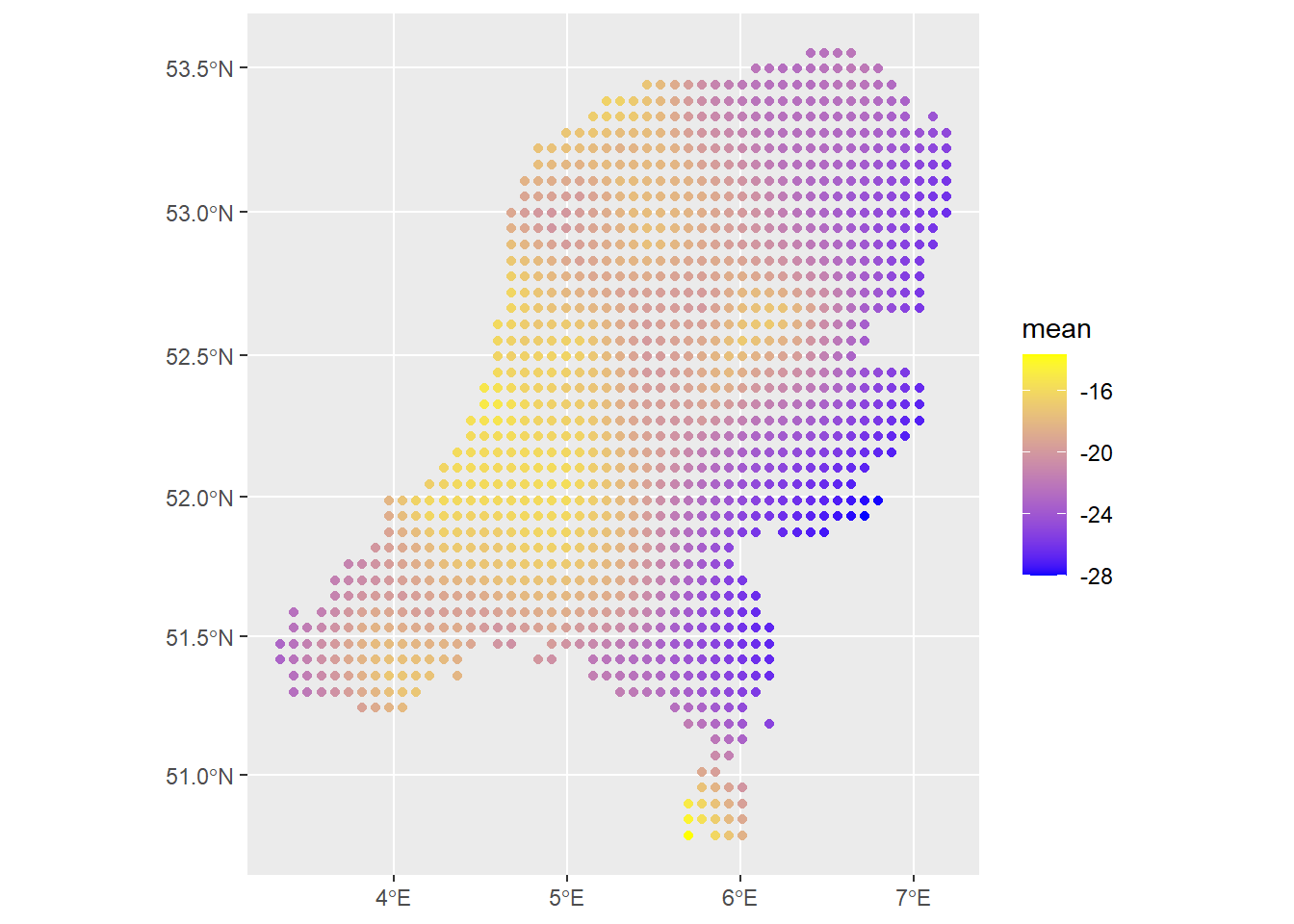

# Check the contribution of just the spatial field
ggplot() +
geom_sf(data=predictions2, aes(color=mean)) +
  scale_colour_gradient(low = "blue", high = "yellow")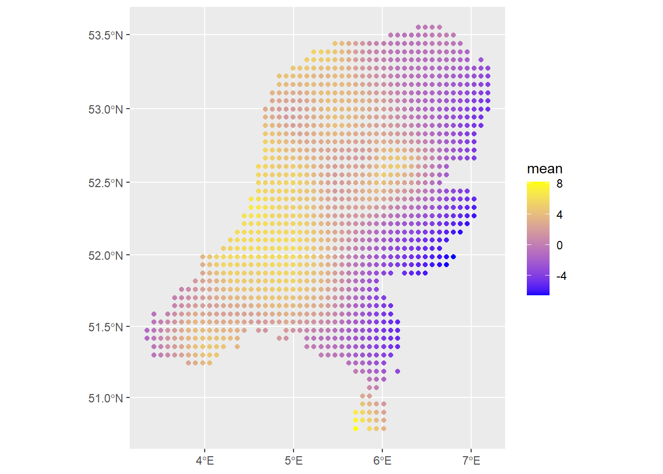

The spatial field looks reasonable. The estimated values of the intensity are so small because we are working on the scale of meters and there are not that many observations, so per meter we do not expect the intensity to be very strong, i.e., it is not very likely for a point observation to occur within any square meter. We can get better resolution and a smoother field if the number of prediction points is higher. I observed that the PC prior for the range of the matern covariance structure \(\rho\) has quite an effect, especially since there are no covariates here. That’s another thing to look out for in your own applications.

That concludes my demonstrations using the INLA and inlabru software. This may hopefully serve as a useful reference for someone, that someone being at least myself. As can be seen, the INLA modelling approach is quite flexible and can be used to construct all sorts of models. Constructing the model isn’t the easiest thing in the world though, and understanding each element can take a while. But the advantage is that once you are comfortable with it, there is a lot that can be done all under the same INLA umbrella. inlabru is a lot easier to use than INLA but it makes some assumptions under the hood that may be advantageous from a statistical perspective (more efficient, robust), but wave away some of the important complexity and the connection of the software to the method of INLA itself. In the end, this blog post was more about INLA than it was about LGCPs, but one begets the other and so it was the natural order of things.

Simpson, Daniel, Håvard Rue, Andrea Riebler, Thiago G. Martins, and Sigrunn H. Sørbye. 2017. “Penalising Model Component Complexity: A Principled, Practical Approach to Constructing Priors.” Statistical Science 32 (1): 1–28. https://doi.org/10.1214/16-STS576.

Simpson, D., J. B. Illian, F. Lindgren, S. H. Sørbye, and H. Rue. 2016. “Going Off Grid: Computationally Efficient Inference for Log-Gaussian Cox Processes.” Biometrika 103 (1): 49–70. https://doi.org/10.1093/biomet/asv064.